Your browser (Internet Explorer 6) is out of date. It has known security flaws and may not display all features of this and other websites. Learn how to update your browser.
X
Design for the ideal text editor.

Design for the ideal text editor

Update: There is now a RFC for Swiboe defining this design in more detail. Comments welcome.

Last time I discussed my thoughts on the ideal text editor. I also mentioned that nothing quite fits the bill for me right now. Today, I want to discuss a possible design for an editor that I think allows for all the things that I look for and that is future proof.

I put a lot of thought into this lately - my frustration with Vim's shortcoming's in daily life and my experiences in writing one of the more successfull Vim plugins out there have given me some insights which I tried to distill in this design. I am currently exploring these ideas in code in Swiboe - my attempt at implementing the editor of by dreams. Contributions are welcome.

The best editor is no editor at all

A simple idea got me started: everything is a plugin and a plugin has infinite power. In Swiboe, these are all plugins: the buffer management (editing, creating, loading), the fuzzy searcher, the git integration, the GUI program, the cursor handling in the gui, the plugin loading - every functionality. Swiboe is really just an operator on a switchboard:

Switchboard operator. Image curtsey of Wikipedia.

That is where its name is coming from: Switch Board Editor.

But how does that work? Let's design two basic plugins that know how to open compressed files into buffers, one that can read Gzip, one that can read Bzip.

Swiboe listens on a socket and waits for plugins to connect. Once a plugin connects, it registers remote procedure calls (RPCs) which have a name and a priority.

# In gzip.py
plugin = connect_to_swiboe("/var/run/swiboe.socket")
plugin.register_rpc("buffer.open:gzip", priority = 800, buffer_open_gzip)

# In bzip.py
plugin = connect_to_swiboe("/var/run/swiboe.socket")
plugin.register_rpc("buffer.open:bzip", priority = 799, buffer_open_bzip)

We'll define the buffer_open_gzip function later - buffer_open_bzip follows by analogy.

Some other client (for example the GUI) now wants to open a file:

gui = connect_to_swiboe("/var/run/swiboe.socket")
gui.call_rpc("buffer.open", args = {
   "uri": "file:///tmp/somefile.txt.gz"
})

The args will be converted to JSON and handed to the called function.

The name of the called RPC defines what will get called: Swiboe will find all registered RPCs that have the same prefix, so in our case both buffer.open:gzip and buffer_open:bzip match. The name of the RPCs are really just a convention: dot.separated.namespaces:name_of_implementing_plugin. This allows callers to call to a very specific function:

# I know that somefile.txt.bz is really a gzip file, so call the gzip
# handler directly. Signal it through 'i_know_what_i_am_doing' that we are
# aware that the extension does not match.
gui.call_rpc("buffer.open:gzip", args = {
   "uri": "file:///tmp/somefile.txt.bz",
   "i_know_what_i_am_doing": True,
})

It also allows to call a very broad range of functions:

# Call all buffer functions that start with o - that is not very useful
# probably.
gui.call_rpc("buffer.o", args = {
   "uri": "file:///tmp/somefile.txt.bz",
})

After the functions are determined, Swiboe sorts them by priority and tries them one after the other. The functions work like event handlers in JavaScript or GUIs - they can choose to handle the call and return a value, or they can let the call through to the next. For example, the gzip handler could look like this:

import gzip

def buffer_open_gzip(rpc_context, uri, i_know_what_i_am_doing = False):
   if not uri.endswith(".gz") and not i_know_what_i_am_doing:
      # Let's inform Swiboe that we do not know what to do with this
      # request.
      return rpc_context.finish(NOT_HANDLED)
   file_path = uri[7:]  # Removes file://
   content = gzip.open(file_path).read()

   # Call an RPC to create a new buffer.
   buffer_create_rpc = rpc_context.call_rpc("buffer.create", {
      "content": content,
      "uri": uri,
   })

   # Wait for it to succeed or fail and return this value to our caller.
   return rpc_context.finish(buffer_create_rpc.wait())

Pro: Events are nothing special

This design can also express something like Vim's autocommands - which are just callbacks, really.

A callback is just an ordinary RPC. For example, when the buffer plugin creates a new buffer, it calls on.buffer.created, but does not wait for this call to finish. Everybody interested in buffer creation can just register a matching RPC - with a I_DO_NOT_CARE priority. This signals Swiboe that all these functions can be called in parallel.

If that is not desired, a priority can be specified to decide when to run - if two plugins conflict they can fix their priority values to make things work.

Pro: Extensibility

A plugin is all-mighty in this design. Want to add functionality to buffer.new:core? Just override it with something that has a higher priority and do something else in it. Want to filter out your .gitignore files from fuzzy find? Just write a fuzzy_find.files:git that is called before fuzzy_find:core, calls it directly and filters its results before passing them on. Want to use tab key for every kind of smart content expansion? No problem, just define the order of functions to call and Swiboe will handle it for you.

Everything is a plugin and therefore everything can be changed by other plugins.

Pro: Simplicity

There is only one concept to understand in Swiboe: this layered RPC system. Everything else is expressed through it.

There is a little more to the story - for example RPCs can also stream results. For example the fuzzy files finder uses this to get partial results to the GUI as fast as possible. But the core philosophy is just this one concept.

The big concern: Performance

Swiboe is an RPC system using Unix domain sockets right now. A RPC is more overhead than a simple function call. My benchmark is creating a buffer and immediately deleting it - these are 4 round trips:

client (create request) -> Swiboe
Swiboe (create request) -> buffer plugin
buffer plugin (create response) -> Swiboe
Swiboe (create response) -> client

client (delete request) -> Swiboe
Swiboe (delete request) -> buffer plugin
buffer plugin (delete response) -> Swiboe
Swiboe (delete response) -> client

Quick tangent. This displays well why I choose Swiboe as name. It connects plugins until they found the right partner to talk to, enabling communication with discretion and speed.

This flow takes ~290μs on my system - roughly 500 times slower as doing the same with python function calls. However, I did not try to speed it up in any way yet - both the protocol and the encoding are naive right now.

Also, I believe the RPCs are mainly gluing functionality together. Most computation will be run in the plugins, in separate processes, in parallel. I believe that sufficient performance for a fluent and responsive experience can be reached.

And of course, performance is temporary, design is permanent. So let's start with getting this right first.

Disclaimer

There is a lot of dreaming in this post. There is no python client yet for Swiboe. (Update: no longer true). This design is still subject to change and not completely implemented in Swiboe. There is no gzip or bzip plugin.

Also, the exact design and protocol of the layered RPC system is not written down anywhere yet. (Update: no longer true)

Swiboe is open for contributions! If you want to design a cool text editor with me, feel free to reach out.

The ideal text editor

The Ideal Text Editor

I am a Vim user and have been for more than 15 years now - with short stints to other editors from time to time. I also wrote a popular plugin for Vim - so I understand it's internals better than most. Still, I feel that Vim is showing it's age - and it is hardly the ideal editor.

I also used TextMate for a while. I tried Sublime for a week or so and am trying Atom right now - I am writing this post in it. There is also a new kid on the block (sorta) with Brackets which seems to be very focused on web design. All of them are impressive editors, but all fall short in some ways for me. Here are my musings about the ideal text editor.

Here are the most important properties of an ideal text editor for me, in sorted order.

Free

This includes free as in free-beer and free as in free-speech. I used TextMate for about a year and got plenty annoyed that I was unable to fix bugs since it was closed sourced. The developer loosing interest in the project and basically walking away also kinda sealed it's death. Imagine spending time learning a powertool, just to see it abandoned and left to bit rotting - and there is nothing you can do. TextMate seems to be back after some years now - but I would never set on a closed source editor again.

Being monetary free is important to get people involved. An editor that is just 100% free is less risk to try out than one that you might need to shell out $$$ to use.

Responsive

A text editor must react as fast as I can think. It is not acceptable to wait for simple tasks like switching a tab or running a command. I must never be interrupted while the editor needs to finish some computation - like auto completion results or a make command.

Modal

Vim's best feature is its UI. Modal editing opens up so much more abilities to control functionality. There are alternatives that are really good too - for example a fuzzy selector over all available commands. But even when this feature is available: with normal mode you have the full keyboard available for shortcuts.

It also clearly defines cutting points for what undo/redo/repeat does. And Vim's editing language (e.g. daw - delete a word) is intuitive, precise and quick.

I will never ever consider an editor that does not have strong modal support build in. It is fine if it can be turned off of course - as long as it is not implemented as an afterthought.

Easy to extend

This is a biggy. It should not matter what my main language is - as long as it is turing complete I should be able to add new features to my editor. These features should be arbitrarily powerful and seemlessly integrated, i.e. they should be indistinguishible from build in commands. Atom and Sublime are good examples of editors that get this second part pretty right.

What they both get wrong is the choice of language: Atom is JavaScript and Sublime is Python. If you do not speak the language of your editor out, you are demoted to User status.

Vim does a little better: It has support for Python, Ruby, Lua, Lisp ... you name it. Unfortunately all of these integration are second class: You cannot write a full plugin in either of these languages - you need a fair amount of VimScript to glue it together. And after 7 years of UltiSnips I can confirm that VimScript is no fun to write.

So a good editor should support as many languages as possible and all of them should be first class citizens.

Cross platform

I never work on Windows, but I work on Mac OS and on Linux a ton. I need an editor that runs on both. I think cross platform is also really important to atract people - so Windows support is important too.

Console/Remote editing

I do not enjoy working in console Vim. I like my Editor to support me with a rich GUI and I enjoy that my editor saves whenever I switch to the shell.

Howevr, occasionally I need to remote edit files on a server - I use console Vim there. That is a really important feature for me. But even better would be if I could remote edit the files: having the nice gui on my laptop talk (securely) to the editor core running on the server would be great.

A console GUI is still important, since many people still like to work in the console using tmux to never switch the program they are using. That is cool, and I think an editor should support it.

Beautiful

There, I said it. I stare at my text editor 8 hours per day - it should better look nice.

Collaborative

I love working on documents with others in Google Docs. Every collaborater can edit the document live and sees the cursor and the edit actions of others at the same time. Imagine how cool pairing would be in an editor that supports that nicely and natively.

I know that there are plugins/hacks for existing editors - but it needs to be there out of the box and easy to setup for people to actually pick it up.

Conclusion

These are the things I ask from an editor. I might have forgotten some stuff, but these are the important things. I will continue this series of blog posts with looks at the editors that are currently out and how they fare. Also I want to present a design that I think works to implement an editor close to my heart.

Technology revamp on the blog

Technology revamp

The technology on the blog bit rotted quite a bit lately. And of course it has not seen any update or new content in years, but that is an entirely different story.

To make sure the content still looks good in modern browsers, I revamped some of the tech behind the site a bit now. For starters, I removed Cufon - a library to render fancy texts client side. I did not use it a lot and it made some text on the page look blurred on my phone.

I also switched from pre-rendered images for math display to using MathJax. MathJax is not fully convincing - pretty heavyweight in terms of size, tons of features I do not need and rather slow rendering. But it works well on my phone and desktop and the math looks better than the images did, so I'll stick with it for now.

The alternative I looked at was KaTeX. It is way faster than MathJax, but unfortunately does not support the TeX align environment, which is a show stopper for me.

Text Layouting Status Report

Text Layouting Status Report

So, it took me two weeks to finally get around to a status report, and Peter even had to request it forcefully. But I have not been idle in this time. Let's see.

Pango? Harfbuzz? SDL_TTF!

I spent quite some time investigating Pango and Harfbuzz, I blogged about it in my previous post. I knew back then already that Pango was not ideal and that even Wesnoth was not using Pango for their fancy help rendering (they use if for some other types of text though). I then investigated Harfbuzz further and though it seems like it will one day become what we need, it is not there. In fact, it does not even have a stable version currently released. It can handle international text pretty well, but it does not help in the left-to-right, top-to-bottom rendering of text, nor with the breaking of text into paragraphs.

So we are back to square one: The old-and-trusted SDL_TTF. I designed my code around SDL as graphics engine, the text rendering is kinda plugged in and uses SDL_TTF, but it should be easy to replace this with any other text engine when one establishes itself as the one - be it Pango or Harfbuzz or anything else in the future.

What works?

I just finished my initial implementation of the engine - It has all the feature that Venatrix and myself have marked as desirable. Some of the feature (like tables) are rather rudimentary, but I think it should be enough for us. The whole engine is currently a stand alone library - in the next step, I will plug it into the Widelands code.

But let's move on to pretty pictures. Here are some examples.

<rt>
<sub padding=5 background=000000>
<sub width=350 background=win_bg.png padding=2>
<p align=center>
   <font size=30 color=F2DF91 underline=true>This is a heading</font>
</p>
<vspace gap=2>
<sub margin=5 padding=5 background="ffffff" float=left>
   <p><img src="wl-ico-128.png"></p>
   <p align=center>
      <font size=10>This is the subtext for the image. Kinda like a
      caption.</font>
   </p>
</sub>
<p indent=5>
<font color=FEFE00 size=14>
   Lorem ipsum dolor sit amet, consetetur sadipscing elitr, <font
   italic=true ref="hyperlink">sed diam nonumy</font> eirmod tempor <font
   underline=1 ref="somereference">invidunt ut labore et</font> dolore
   magna aliquyam erat, sed diam voluptua. At vero eos et accusam et justo
   <font bold=true>duo dolores et ea rebum</font>. Stet clita kasd
   gubergren, no sea takimata sanctus est Lorem ipsum dolor sit amet.
</font>
</p>
</sub>
</sub>
</rt>

This code renders to the following picture:

Sample image

This already shows off some of the features: changing fonts inside a paragraph, sub layouts that can float inside the text. Margins and paddings for some elements (though this is not as fully featured as in HTML) and of course images. It also contains a ref attribute for a font tag which makes this part of the text clickable. This will make hyperlinks in the help possible.

Tables are kinda possible as well:

<rt>
<sub width=10></sub><sub width=240>
<p>
<sub width=80 background=638c57><p>Hello</p></sub><space><sub
width=80 background=42deb7><p>Nice</p></sub><space><sub
width=80 background=43f447><p>World</p></sub>
<br>

<sub width=80 background=404542 valign=center><p
   align=center>Upsy</p></sub><space><sub
width=80 background=e21038><p>And more</p></sub><space><sub
width=80 background=0c7e8f valign=center><p>Thats all</p></sub>
<br>

</p>
</sub>
</rt>

Each row is a set of three fixed width cells separated by a <space> tag which expands as needed (in this case not at all). The lines are separated by a linebreak tag <br>. This kinda results in a table with fixed column count and width. Good enough for Widelands I hope:

Something like a table

Bullet point lists are possible as well:

<rt>
<p><font size=20 underline=1>A bullet list</font></p>
<sub padding=10 width=490>
<p>
<sub valign=top><p><space fill=" "><img
   src=bullet.png></p></sub><sub width=450>
<p>
Lorem ipsum dolor sit amet, consetetur sadipscing elitr, sed diam nonumy
eirmod tempor.
</p>
</sub>

<sub valign=top><p><space fill=" "><img
   src=bullet.png></p></sub><sub width=450>
<p>
Lorem ipsum dolor sit amet, consetetur sadipscing elitr, sed diam nonumy
eirmod tempor invidunt ut labore et dolore magna aliquyam erat, sed diam
voluptua. At vero eos et accusam et justo duo dolores et ea rebum. Stet
clita kasd gubergren, no sea takimata sanctus est Lorem ipsum dolor sit
amet.
</p>
</sub>

<sub valign=top><p><space fill=" "><img
   src=bullet.png></p></sub><sub width=450>
<p>
Lorem ipsum dolor sit amet, consetetur sadipscing elitr, sed diam nonumy
eirmod tempor.
</p>
</sub>
</p>

</sub>
</rt>

This uses a lot of sub layouts to achieve the desired result. It does not read very nice, but which markup does? I plan to hide this all in some Lua functions, just as we are already doing for scenarios to make it all nice to use as well. This wall of text renders as

Bullet point list

What's next?

The next step is to integrate this layout engine into Widelands. Caching will be really important here, because rendering with SDL_TTF is very slow. I feel that the technical challenges of getting this engine on board will be surmountable, the one thing I am really not looking forward to is changing all rich texts that we already have to work with the new engine. Especially the hard coded texts inside the source, the files in txts/ and the early campaigns (barbarians and empire) will be a lot of tedious work. I hope some people hop on board to help me out with that.

Soo, expect a branch with this engine soonish on launchpad.

Widelands Marathon Begins

My personal Widelands Marathon

So, I finally handed in my PhD thesis. That does not mean that everything is said and done, there is still an oral examination, a 30 minutes talk and some demonstration stuff to be done. But it means that I am now officially out of my previous job.

That means, before I will start at Google in September, I have around three months to use for whatever I see fit (okay, okay, I also need to find a flat, move, prepare for the oral examination, prepare the demo, and organize a huge celebration. And I have some other obligations remaining). I want to use a lot of time for Widelands in these three months. To keep me on track and motivated, I decided to keep a development diary on this blog.

First Project: Make the Widelands Help awesome

Venatrix, Astuur and others have begun the immense project to write a help for Widelands. I have provided a minimal framework to give buildings a help window via a Lua script in the building's directory. This is already immensely useful and significantly better than no help at all, but it feels rather limited: Widelands text handling and layouting capabilities are rather limited and there is currently no way to document other stuff than buildings. My first project for now is to improve this situation.

Text layouting

Text layouting is a difficult problem, especially when we also consider internationalization (just think chinese for example). I started out by learning the various libraries that are around for this problem. There are two contenders, the fist is Pango, the second harfbuzz.

Pango

Pango is the text layouting engine from the Gnome desktop environment. And it is well suited for this task. Using Cairo for rendering and its own (limited) markup language it is next to trivial to render a UTF-8 string with various languages to a rectangular grid. This is not enough for what I want though: Just think about an image inside a paragraph. Text should flow around it, therefore it needs to be broken into a non rectangular shape. This is not easy with Pango: It does provide a low level API to reflow text independently, but it is awkward and one looses at lot of what Pango is good at (like transparent handling of right-to-left text blocks).

Also, Pango does not allow to choose the TTF font file to use for rendering directly, instead relying on fontconfig to find a suitable system font. In Widelands, we would prefer to feed in our font files ourselves - so we can be sure that it looks the same, no matter what OS is used.

Pango is stable and used in a lot of products like Gnome. It is also what Wesnoth uses for most of its rendering needs. But for the (cool) Wesnoth help, it is in fact not used, likely because of the reflow problem I mentioned earlier.

Documentation for Pango is available in the form of a Doxygen output. This is a nice reference, but hardly more useful than the source code itself. There is also no easy tutorial that goes beyond the PangoLayout example that can only render in rectangles. Especially, there is no example how to add custom markup tags or how to do low(er) level layouting. The best I found is an old mailing list post that explains the steps needed to layout text oneself. I was able to stitch those hints together to a binary that does just that. But it is really awkward and it does not offer a lot of the functionality that the PangoLayout wrapper offers. I kinda feel this is a dead-end for now.

Harfbuzz

Harfbuzz is a slightly lower level API that is in fact used by Pango. It allows to load TTF directly and offers more control over layouting. For rendering it also uses Cairo. Problem here is that there is no stable version - according to the homepage, the API might change till 1.0, the current version is 0.6. And there is no docu. Nada!

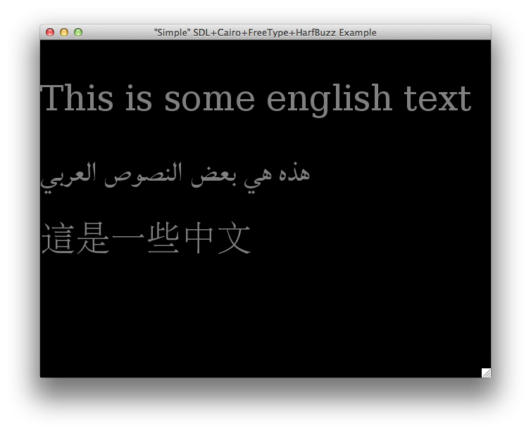
Luckily, there is a github user that provided an example that is very close to what I want to achieve and that shows off a lot of the features of harfbuzz. The API changes were already felt in this one year old example: some of the functions take other arguments now than they did back then, but it was really easy to figure out with the harfbuzz source code nearby. When run, the program shows the following window:

text

I am yet unaware if harfbuzz is also able to break text according to grammatic rules, but this looks promising.

Alright, so far for my two hours of Widelands for today.

Fourth episode of UltiSnips Screencast

UltiSnips Screencast Episode 4

I got around doing the final episode of my little screencast series on UltiSnips. This time I talk about Python interpolation and give an example of a snippet that really makes my life easier.

I always wanted to have a few screencasts showing off the main features of UltiSnips but nobody was willing to take the time and effort to produce them. Now that I've done it myself I can understand why: It takes a lot of time. From start to finish - planing, recording, cutting, uploading and promoting one screencast of roughly ten minutes takes approximately six to eight hours. It was a lot of fun doing the casts though and I learned a lot. I am also reasonably pleased with the final results.

If someone suggest a really good topic for a fifth screencast, I will consider making one. But I feel that UltiSnips' main features are well covered now. Thanks for sticking with me throughout the series!

Third episode of UltiSnips Screencast

UltiSnips 2.0 and Screencast Episode 3

I just release UltiSnips 2.0 together with a short screencast to run you through the new features.

2.0 is a killer-feature release for me: Having normal mode editing and $VISUAL support adds a lot of value to UltiSnips for me.

UltiSnips now has all the features I initially expected from a snippet plugin when I started out writing it. It was not an easy road getting here but I am proud what we have achieved. I consider it now mostly feature complete - I will not object to good ideas for new features that enhance the user experience but we will try as best as we can to avoid feature creep. UltiSnips wants to be only one thing - the ultimate solution for snippets in Vim.

The Statistical View on Least Squares

Least Squares and Statistics

Last time I talked about the beautiful linear Algebra interpretation of Least Squares which adds a wonderful geometric interpretation to the analytical footwork we had to do before. This time I will borrow from a video I saw on Khan Academy a long time ago. I connects some of the elemental principles of statistics with regression.

The basic idea is similar to the analytical approach. But this time, we will only try to fit a line to $$M$$ $$x$$/$$y$$ pairs. So, we have a model of the form

\begin{equation*}y(x) = m x + c.\end{equation*}

The squared errors between model and data is then

\begin{align*}S := \sum_i \epsilon_i^2 &= \sum_i (m x_i + c - y_i)^2 \\ &= \sum_i m^2 x_i^2 + 2 c m x_i + c^2 - 2 m x_i y_i - 2 c y_i + y_i^2\end{align*}

Of course, we search for the global minima of this solution with respect to the parameters $$m$$ and $$c$$. So let's find the derivations:

\begin{align*}0 \stackrel{!}{=} \frac{\partial S}{\partial m} &= \sum_i 2 m x_i^2 + 2 c x_i - 2 x_i y_i \\ 0 \stackrel{!}{=} \frac{\partial S}{\partial c} &= \sum_i 2 m x_i + 2 c - 2 y_i\end{align*}

We can conveniently drop the 2 that appears in front of all terms. We will now rewrite these equations by using the definition of the sample mean:

\begin{equation*}\overline{x} = \frac{\sum_i x_i}{M}\end{equation*}

This gives:

\begin{align*}0 \stackrel{!}{=} m M \overline{x^2} + M c \overline{x} - M \overline{x y} \\ 0 \stackrel{!}{=} m M \overline{x} + M c - M \overline{y}\end{align*}

Let's loose the $$M$$ s and solve for $$m$$ and $$c$$.

\begin{align*}m &= \frac{\overline{x}\,\overline{y}- \overline{x y}}{\overline{x}^2 - \overline{x^2}} \\ c &= \overline{y} - m \overline{x}\end{align*}

If you look closely at the term for the slope $$m$$ you see that this is actually just the covariance of $$x$$ and $$y$$ divided by the variance of $$x$$. I find this very intriguing.

Second episode of UltiSnips Screencast

UltiSnips Screencast Episode 2

Second screencast is done and ready! If you have not yet seen the first, look over here. This was done under the maxim Done is better than perfect. I had more advanced explanations planed, but the screencast turned out to be longer than expected. I therefore opted for a complete overview over the most common features of UltiSnips and will explain some cooler stuff in this blog post.

So here is the video. You can find some snippets with their explanation below.

Elements inside of default text

Placeholders can contain other UltiSnips elements. This is totally cool and very useful. For example, the following snippet is defined for the html file type and ships with UltiSnips:

snippet a
<a href="$1"${2: class="${3:link}"}>
    $0
</a>
endsnippet

It allows to either delete the complete tabstop 2 with one keystroke. Or you can jump to tabstop 3 and replace the CSS class name.

Another example:

snippet date
${2:${1:`date +%d`}.`date +%m`}.`date +%Y`
endsnippet

This snippet will enter the current date in the format that is used in Germany: dd.mm.yyyy. Jumping forward will allow you to either overwrite the day or the day and the month. I use this in my todo files to enter due dates.

Complete Scripts in Shell Interpolation

Shell interpolation is as powerful as the shell itself. Here is a silly example that is basically a complete Perl script:

snippet random
`#!/usr/bin/perl
use LWP::Simple qw(get);
my $page = get "http://www.random.org/integers/?num=1&min=1&max=100&col=1&base=10&format=plain&rnd=new";
print $page`
endsnippet

This snippet will insert a truly random number between 1 and 100 fetched from random.org. Useful? Maybe not, but a good example.

Transformations are more powerful than you might think

This transformation shows the transformation option g which means global replace. It will uppercase every word in the first tabstop while mirroring its content.

snippet title "Titelize in the Transformation"
${1:a text}
${1/\w+\s*/\u$0/g}
endsnippet

In the replacement part of this transformation, the u means "uppercase the next character" and the $0 matches everything found. The complete transformation basically says: find a word \w+ and any number of whitespace \s* and replace them through what you found, but uppercase one char. The g at the end makes sure that not only the first but all words are uppercased.

Conditional replacements

One feature that I didn't mention in the screencast are conditional replacements. When you capture a group in the search part of a replacement, you can check if it was matched in the replacement like so: (?<number>:yes text:no text). yes text will be inserted if the group was matched, otherwise no text will be inserted. A quick example:

snippet cond
${1:some_text}${1/(o)|(t)|..*/(?1:ne)(?2:wo)/}
endsnippet

The transformation will match a o at the beginning into group 1 or a t at the beginning in group 2. The rest of the search string just matches everything of the first tabstop. The replacement will either be ne when a o was matched, wo when a t was matched or an empty string. That means that you can just type a t to quickly get two as the complete content of the snippet or a o to get one. If you type anything else, you only get the content of the place holder, i.e. the verbatim of what you typed.

Inword triggers

The snippet option 'i' stands for inword trigger. Let's say for some coding project, I often want to get variables that end on izer: maperizer, vectorizer... I want to define a snippet with ri which should expand to izer. Triggers are always matched to full words though - except for when you use the i option for your snippet:

snippet ri "rizer" i
rizer
endsnippet

This does what I want: maperi<tab> -> maperizer.

Regular Expression triggers

Regular expression triggers can be used with the r option to a snippet. Note that you have to add delimiters around your trigger when using regular expression triggers. I use the following snippet because I can never remember on which exact trigger I set my $$\textrm{\LaTeX{}}$$ chapter snippet:

snippet "chap?t?e?r?" "Latex chapter" rb
\section{chapter}
   $0
\end{chapter}
endsnippet

This will expand on either cha, chap, chapt, chapte or chapter. Regular Expression triggers are even more powerful because you can get access the to match object inside your python interpolation blocks. More on that in the next episode.

Regular expression triggers also allow to define triggers with special characters, whitespace or multi word triggers.

snippet " this is a trigger" "Multiword & Whitespace" r
Hello World
endsnippet

Conclusion

The features we discussed so far are enough to make crazy snippets and will suffice for most uses. If you ever feel lost or forget how to use one of the features, take a look into UltiSnips help document, either via

:help UltiSnips

or here online.

Next time we will discuss python interpolation which brings even more power to snippets. With it, some of the features we discussed so far will become easier to read with and others will only then become possible. With python interpolation there is basically nothing that a snippet can't do.

As always, leave comments and let me know what you think about the screencast and the tips. Also let me know what you are interested in and what you would like to see in future screencasts. I have no more topics for a fourth screencast, so if you want one, let me know what you want to see in it.

Move window done right

Move window to the rescue

Overlapping windows are a bad invention. Frankly, the one UI that works are virtual desktops with non overlapping windows (e.g. window managers). Given, the world becomes sane slowly with iOS leading the way: every application is full screen there.

On Mac OS X, the situation is dire: windows just open wherever they want to. I wrote a python script a while ago that can be called quickly from Quicksilver or LaunchBar which took a simple syntax to describe where you want your window and moved it there. Problem: it was rather slow. It needed to run and parse a command line tool to get number of screens and resolutions and it had to ask for the frontmost application via AppleScript.

I got fed up with that yesterday and made it fast. Getting the frontmost application and the number of screens and their resolution is now done via the Carbon Framework in a C Extension. You can find the source code on GitHub, download from there and use pip to install:

https://github.com/SirVer/move_window

Usage

You want to call this from LaunchBar or Quicksilver, so install/make a proper AppleScript (I ship one in contrib). The tool takes the following syntax:

move_window <screen_id><nr of x parts><x span><nr of y parts><y span>

Some examples

move_window 0     # Disp 0, full Screen
move_window 02    # Disp 0, left half of screen
move_window 030   # Disp 0, left third of screen
move_window 031-2 # Disp 0, rightmost two thirds of screen
move_window 12121 # Disp 1, bottom right quarter of screen

Feedback and pull request are very welcome!

First episode of UltiSnips Screencast

UltiSnips Screencast Episode 1

I finally got the technicalities sorted out, some inspiration and the time to make a first screencast about UltiSnips. It is not so much about the specifics in UltiSnips but rather an overview what snippets are and a demo reel of some of UltiSnips features.

Let me know in the comments what you would like to see in future episodes!

Update: There is now a second screencast.

The Linear Algebra View on Least Squares

A Linear Algebra View on Least Squares

Last time, we introduce the least squares problem and took a direct approach to solving it. Basically we just minimized the $$y$$-distance of a model to the data by varying the parameters of the model. Today, we find a completely different, but very neat interpretation.

Suppose we have the following problem: There is a set of linear equations without a solution, e.q. a matrix $$\mat{A}$$ and a vector $$\vec{b}$$ so that no vector $$\vec{x}$$ exists that would solve the equation.

\begin{equation*}\mat{A} \vec{x} = \vec{b}.\end{equation*}

Bummer. What does that actually mean though? If we use every possible value of $$\vec{x}$$ in this equation, we get essentially all linear combinations of the column vectors of $$A$$. That is a span of vectors. That is a subspace. So, $$\vec{b}$$ is not in our subspace, otherwise we would find an $$\vec{x}$$ that would solve our linear equation.

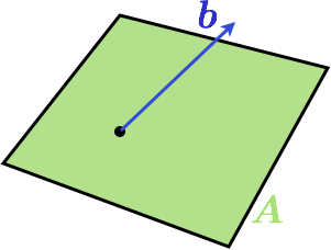
Here is a visualization in 3D when A is a two dimensional matrix:

2D Matrix with Vector not in its Column Space

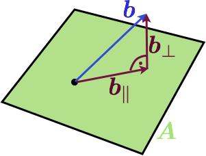
The column space of the matrix is a plane and $$b$$ is not in the plane. A natural question now is: what is the vector in the column space of $$\mat{A}$$ that is the best approximation to $$b$$. But what is a good approximation? Well, how about the Euclidian distance between the endpoints of the vectors. If we choose this criteria, there is a simple solution: the projection of $$\vec{b}$$ to $$\mat{A}$$ will give the best approximation. Here is another image:

Image with projected vectors

We have decomposed $$\vec{b}$$ into its best approximation in $$\mat{A}$$ which we call $$\vec{b_\parallel}$$ and a component that is orthogonal to it called $$\vec{b_}\perp$$. At the end of the day, we are interested in a best approximated solution to our original equation, so we are not really interested in finding $$\vec{b}_\parallel$$, but rather an $$\vec{x^*}$$ so that

\begin{equation*}\mat{A} \vec{x}^* = \vec{b}_\parallel\end{equation*}

Lets look for an equation for this $$\vec{x}^*$$. We will start out by using that the two components of $$\vec{b}$$ are perpendicular to each other. And we will also express $$\vec{b}_\perp$$ through vector addition.

\begin{align*}0 &= \vec{b}_\parallel ^T \vec{b}_\perp \\ &= (\mat{A} \vec{x}^*)^T \vec{b}_\perp \\ &= (\mat{A} \vec{x}^*)^T (\vec{b} - \mat{A} \vec{x}^*) \\ &= \vec{x}^{* T} \mat{A}^T (\vec{b} - \mat{A} \vec{x}^*) \\ &= \vec{x}^{* T} ( \mat{A}^T \vec{b} - \mat{A}^T \vec{A} \vec{x}^*)\end{align*}

Since $$\vec{x}^*$$ can't be zero, the term in parenthesis must be. This directly yields the least squares formula again:

\begin{equation*}\vec{x}^* = (\mat{A}^T \mat{A})^{-1} \mat{A}^T \vec{b}\end{equation*}

Conclusion

We did the exact same thing as in the last post, but this time we took another approach and quite a different world view on the problem. The least squares solution came up very naturally here and with a very simple geometric interpretation (at least in the 3d case, the approach is also valid for other dimensions though).

The last iteration of this series will take a look at least squares in statistical models.

A direct look on least squares

Least squares

Here we go again. After a long time of travelling and illness something new on this blog. Today, I start a new mini series that takes a look at Least Squares in various ways. I want to show how least squares arises naturally in various areas - of course this will look at little similar all the time because it stays the same principle; but the basic approach depends on the context.

Today we start with a simple example and the method I'll call the direct approach.

The direct method

Suppose we have some kind of measurement process that measures every second and we know that the system we measure follows a model of third order, that is the values we expect are

\begin{equation*}m(t) = p_1 t^2 + p_2 t + p_3.\end{equation*}

But obviously, our measurement process is in some way noisy. Our aim is now to find good values for $$p_1, p_2$$ and $$p_3$$. But what is good? Well, why not start by minimizing the distance between our model prediction and the measurement values?

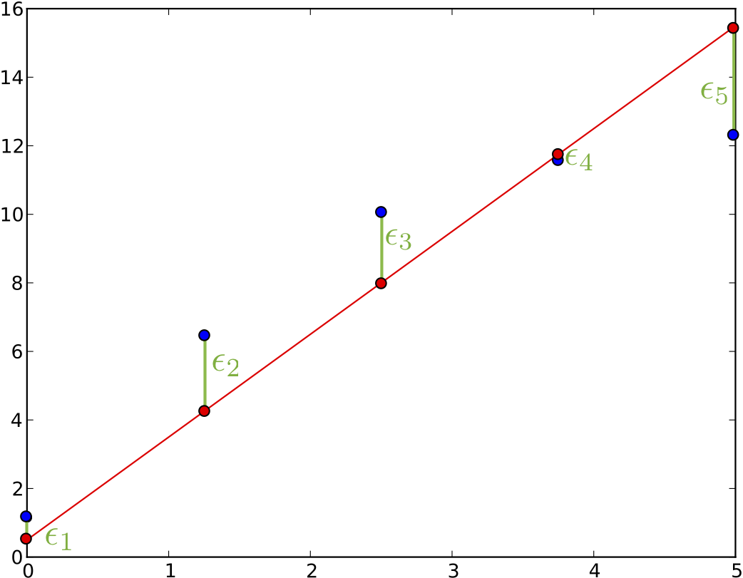
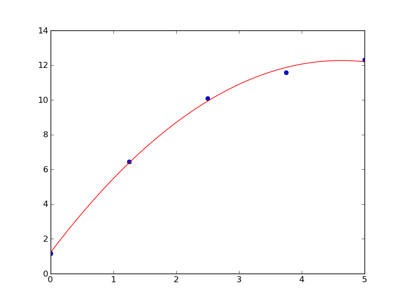
First plot showing a bad model fit and the errors we want to reduce.

In this plot we see our measurements as blue dots and we see an awful model fit as red line. And we see various $$\epsilon$$ bars. Those are the errors we want to minimize, the model prediction at a point $$t_i$$: minus the value that we measured at this point $$v_i$$:

\begin{equation*}\epsilon_i = m(t_i) - v_{i} = p_0 t_i^2 + p_1 t_i + p_3 - v_i = \begin{pmatrix} t_i^2 & t_i & 1 \end{pmatrix} \begin{pmatrix} p_1 \\ p_2 \\ p_3 \end{pmatrix} - v_i\end{equation*}

It seems like a bit of a stretch to write this simple equation in a matrix notation there in the last step. But it will benefit us in a moment.

We do not want to minimize the straight sum of those because positive and negative values might zero out. The absolute value is also not so easy because our error function is then non-smooth... Let's summarize the sum of squares of the individual errors:

\begin{equation*}S := \sum_{i=1}^5 \epsilon_i^2\end{equation*}

Minimization is best when we have a quadratic error function because there is only a single global minimum which can be found by setting the gradient to zero.

The notation of this minimization becomes a bit tedious, that's why we go back to the matrix notation we used earlier and realize that we can stack all measurements we have into one matrix. Working with vectors will make the derivatives easier to do:

\begin{align*}\vec{\epsilon} &= \begin{pmatrix} m(t_1) - v_1 \\ \vdots \\ m(t_5) - v_5 \end{pmatrix} \\ &= \begin{pmatrix} p_1 t_1^2 + p_2 t_1 + p_3 - v_1 \\ \vdots \\ p_1 t_5 ^2 + p_2 t_5 + p_3 - v_5 \end{pmatrix} \\ &= \underbrace{\begin{pmatrix} t_1^2 & t_1 & 1 \\ \vdots \\ t_5 ^2 & t_5 & 1 \end{pmatrix}}_{:= \mat{M}} \underbrace{\begin{pmatrix} p_1 \\ p_2 \\ p_3 \end{pmatrix}}_{:= \vec{p}} - \underbrace{\begin{pmatrix} v_1 \\ \vdots \\ v_5 \end{pmatrix}}_{:= \vec{v}}\end{align*}

Our error function $$S$$ then becomes

\begin{align*}S & = \vec{\epsilon}^T \vec{\epsilon} \\ &= (\mat{M} \vec{p} - \vec{v})^T (\mat{M} \vec{p} - \vec{v}) \\ &= \vec{p}^T \mat{M}^T \mat{M} \vec{p} - \vec{p}^T \mat{M}^T \vec{v} - \vec{v}^T \mat{M} \vec{p} + \vec{v}^T \vec{v}\end{align*}

Finding the gradient of S with respect to the parameter vector $$\vec{p}$$ is now easy. We also immediately set this equal to the zero vector to find the minimum of this function:

\begin{equation*}\nabla S = 2 \mat{M}^T \mat{M} \vec{p} - \mat{M}^T \vec{v} - \mat{M}^T \vec{v} \stackrel{!}{=} \vec{0}\end{equation*}

And so we find the parameters that minimizes the error to be

\begin{equation*}\vec{p} = (\mat{M}^T \mat{M})^{-1} \vec{M}^T \vec{v}\end{equation*}

Using this with the above example we get the following best fit

Best fit for the model

Conclusion

I call this the direct approach because we directly set out to minimize the quantity and the least square formula pops out. There are other goals one can set out to achieve which leads to the same formula which I will show in some of the next posts. Hopefully it will not take as long again till I find some time to post again.

The bridge between Lagrange and Bezier interpolation

Comparing Lagrange and Bezier interpolation

Let's continue our discoveries in Chapter 7 of the Book by discussing my solution to 7.P1.

We have talked the de-Casteljau algorithm before. It is an expensive but numerically stable way to calculate the points on a Bézier curve given it's control Polgon. Just to remember, this is how it is calculated:

Given the points $$\vec{b}_0 ... \vec{b}_n \in \mathbb{R}^m$$, $$t \in \mathbb{R}$$. Set

\begin{eqnarray*}\vec{b}_i^0(t) & := & \vec{b_i} \\ \vec{b}_i^r(t) & := & (1-t) \vec{b}_i^{r-1}(t) + t\,\vec{b}_{i+1}^{r-1}(t)\end{eqnarray*}

Then $$\vec{b}_0^n(t)$$ is the point with the parameter $$t$$ on the corresponding Beziér curve.

Another common approach to interpolation is to use Polynoms of degree $$n$$. We than also need some $$t_i \in \mathbb{R}$$ that corresponds to the given $$\vec{b}_i$$, if they aren't given we can just set them so that they are equally distributed betwenn $$[0,1]$$.

Aitken's Algorithm is than defined by

Given the points $$\vec{b}_0 ... \vec{b}_n \in \mathbb{R}^m$$, with corresponding $$t_i \in \mathbb{R}^n$$ and the position of the interpolation $$t \in \mathbb{R}$$. Set

\begin{eqnarray*}\vec{b}_i^0(t) & := & \vec{b_i} \\ \vec{b}_i^r(t) & := & \frac{t_{i+r} - t}{t_{i+r} - t_i} \vec{b}_i^{r-1} (t)+ \frac{t - t_i}{t_{i+r} - t_i}\,\vec{b}_{i+1}^{r-1}(t)\end{eqnarray*}

Then $$\vec{b}_0^n(t)$$ is the point with the parameter $$t$$ on the corresponding interpolating Polynom.

The geometric interpretation is the following: We start out with point 0 and 1 and interpolate linearly between them, than we take 1 and 2 and so on. In the next step, we linearly interpolate between the linear interpolations of the last round by blending the one into the other. The degree of the interpolation polynom increses in each step by one.

The differences between de-Casteljau and Aitken's algorithm in each step are quite simple: The first one is a mapping from $$[0,1] \to \mathbb{R}^m$$ while the second one is mapping from $$[t_i, t_{i+r}] \to \mathbb{R}^m$$.

We can provide a straight forward combination of those two algorithms by mapping from the interval $$[ 0\alpha + (1-\alpha) t_i, 1 \alpha + (1-\alpha) t_{i+r} ]$$ with an $$\alpha \in \mathbb{R}_+$$, that is, we linearly interpolate between the two intervals. Let's define a quick helper function:

\begin{equation*}W_i^r(t) := \frac{\alpha + (1-\alpha) t_{i+r} - t}{\alpha + (1 - \alpha) (t_{i+r} - t_i)}.\end{equation*}

Using this, the generalized algorithm looks like this

Given the points $$\vec{b}_0 ... \vec{b}_n \in \mathbb{R}^m$$, with corresponding $$t_i \in \mathbb{R}^n$$, a blending factor $$\alpha \in \mathbb{R}$$ and the position of the interpolation $$t \in \mathbb{R}$$. Set

\begin{eqnarray*}\vec{b}_i^0 (t) & := & \vec{b_i} \\ \vec{b}_i^r(t) & := & W_i^r(t) \vec{b}_i^{r-1}(t) + (1 - W_i^r(t))\,\vec{b}_{i+1}^{r-1}(t)\end{eqnarray*}

Then $$\vec{b}_0^n(t)$$ is the point with the parameter $$t$$ on the corresponding blend between Bézier and Polynomial interpolation.

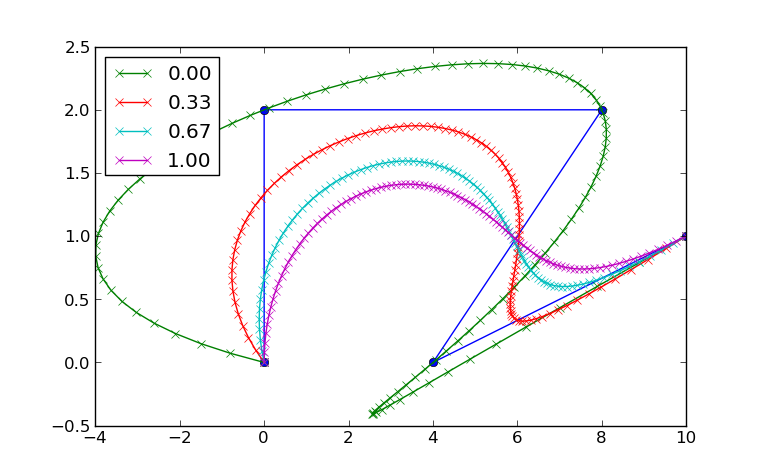
The De-Casteljau algorithm is the special case for $$\alpha = 1$$, Aitken's Algorithm is the special case for $$\alpha = 0$$. Here is a plot of a planar interpolation:

Blending between Lagrange and Bezier with various values of alpha

See how the curve for $$\alpha = 0$$ passes through all 4 points. This is a property of Lagrange interpolation (polynomial interpolation). The curve for $$\alpha = 1$$ is the only one that stays in the convex hull of the points; this is a property of Bézier curves.

As always, you can find the complete code for this post in the GitHub repository under chap07. Also, Farin has written a paper on this very topic. You can find it here.

Better Navigation

Better Navigation on this Blog

I just added a calendar widget on each page where it makes sense here. I am not sure how useful it is, so I will try it out for a while and remove it again if it makes no sense.

I also improved the blog archive list in the right navigation bar. I was inspired by something I saw on Guido's blog, namely a folding tree view. I am aware that most blogging tools like Wordpress have this feature build in, but I realized the first time how useful it is on Guido's page. So I copied it. Turned out that you only need a little bit of Javascript and CSS. I basically followed the short but concise tutorial by David Herron. I only needed very few adjustments, but they were trivial thanks to the beauty that is jQuery.

Degree Reduction of Bezier Curves

Degree Reduction of Bezier Curves

Continuing with my reading efforts in Curves and Surfaces for GACD by Gerald Farin, I will talk today about a topic that comes up in chapter 6: elevating and reducing the degree of a Bézier curve.

Elevating the dimensionality

First, we start out by proving that the degree of a Bézier curve can always be elevated without the curve being changed.

A curve $$\vec{x}(t)$$ with the control polygon $$B = {\vec{b}_0, \ldots, \vec{b}_n}$$ can be represented as a Bézier curve using the Bernstein Polynomials $$B_i^n$$ as basis:

\begin{equation*}\vec{x}(t) = \sum_{i=0}^{n} \vec{b}_i B_i^n(t)\end{equation*}

We will now prove that we can increase the degree from $$n$$ to $$n+1$$ and still keep the same curve, given we choose then new control polygon accordingly.

We start out by rewriting $$\vec{x}(t)$$ as

\begin{eqnarray*}\vec{x}(t) &=& (1-t) \vec{x}(t) + t \vec{x}(t) \\ &=& \sum_{i=0}^n (1-t) \vec{b}_i B_i^n (t) + \sum_{i=0}^n t \vec{b}_i B_i^n (t)\end{eqnarray*}

And now we show that the terms can be rewritten as a sum from 0 to n+1. Let's start with the first term:

\begin{eqnarray*}(1-t) B_i^n (t) &=& (1-t) \frac{n!}{(n-i)! i!} t^i (1-t)^{n-i} \\ &=& \frac{n + 1 - i}{n + 1} \frac{(n+1)!}{(n+1 -i)! i!} t^i (1-t)^{(n+1)-i} \\ &=& \frac{n+1 - i}{n+1} B_i^{n+1}(t)\end{eqnarray*}

Easy. Now the second one

\begin{eqnarray*}t B_i^n(t) &=& t \frac{n!}{(n-i)! i!} t^i (1-t)^{n-i} \\ &=& \frac{i+1}{n+1} \frac{(n+1)!}{(n+1)!(i+1)!} t^{i+1} (1-t)^{n-i} \\ &=& \frac{i+1}{n+1} B_{i+1}^{n+1} (t)\end{eqnarray*}

Now, we plug this into the summation formula. We can readjust the summation variables cleverly by noting that we only add 0 terms and we get the formula:

\begin{eqnarray*}\vec{x}(t) &=& \sum_{i=0}^{n+1} \frac{n+1-i}{n+1} \vec{b}_i B_i^{n+1} (t) + \sum_{i=0}^{n+1} \frac{i}{n+1} \vec{b}_{i-1} B_i^{n+1} (t) \\ &=& \sum_{i=0}^{n+1} \Big( \big(1 - \frac{i}{n+1}\big) b_i + \frac{i}{n+1} b_{i-1}) \Big) B_i^{n+1} (t)\end{eqnarray*}

Now all there is to do is to compare the coefficients for old control polygon points and new polygon points and we have our solution: the new points are linear interpolations of the old ones. We can find the new points $$\vec{B}^{(1)}$$ from the old $$\vec{B}$$ by a simple Matrix multiplication:

\begin{equation*}\mat{M} \vec{B} = \vec{B^{(1)}}\end{equation*}

with the Matrix $$\mat{M}$$ being of shape $$n+1 \times n$$ and looking something like this:

\begin{equation*}\mat{M} = \begin{pmatrix} 1 & & & \\ \frac{1}{n+1} & 1- \frac{1}{n+1} & & \\ & \frac{2}{n+1} & 1- \frac{2}{n+1} & \\ \vdots \\ & & \frac{n}{n+1} & 1- \frac{n}{n+1} & \\ & & & 1 \end{pmatrix}\end{equation*}

Degree Reduction

The hard work is already done now: It only remains to say that we indeed find the best approximation to our Bézier curve (in the least squares sense) by finding the least-squares solution to the inverse of the system of equations given in the Matrix equation. Therefore, we find the best degree reduced control polygon by

\begin{equation*}\vec{B} = (\mat{M}^T \mat{M})^{-1} \mat{M}^T \vec{B}^{(1)}\end{equation*}

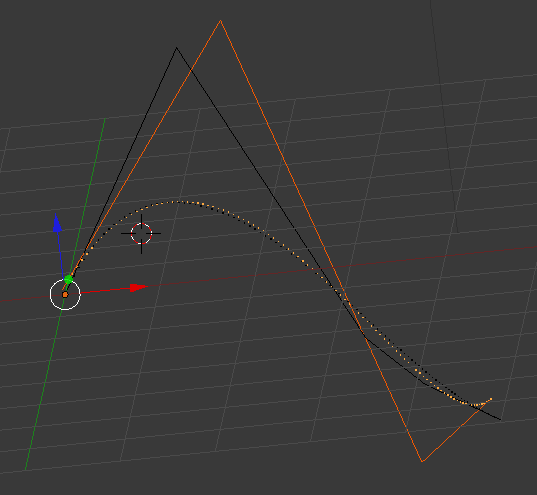
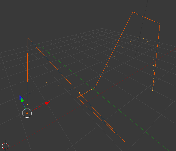
And here is an example from inside Blender. The highlighted objects are the reduced control polygon (n=4) and its Bézier curve. The non highlighted are the originals with one degree higher (5).

Reduced control Polygon and original + splines

As always, you can find the source code for this in the corresponding GitHub project.

Generators in C++

Generators in C++

Generators are iterators over things made up on runtime. For example if you ask me about the Fibonacci sequence, I can generate an infinite amount of them by only remembering the two numbers before:

\begin{eqnarray*}F(0) &=& 1 \\ F(1) &=& 1\\ F(n) &=& F(n-1) + F(n-2)\\\end{eqnarray*}

Generators are quite useful for programming. Python has them, Haskell is basically build around them (I think they call them infinite lists). Generating the Fibonacci sequence up to a maximum number maxn looks like this in Python:

def fib(maxn):
    n, ln = 1, 1
    while n < maxn:
        yield n
        n, ln = ln, n + ln

for i in fib(1000):
    print i,

After my last blog post about C++0x features, I was intrigued to write something similar in C++. The corresponding main function also looks very nice with the new container iterate feature:

#include <iostream>

int main(int, char argv**)
{
   FibonacciGenerator k(1000);

   for(auto i : k)
      std::cout << i << " ";
   std::cout << std::endl;

   return 0;
}

So basically, we have a container here called FibonacciGenerator and we iterate over it with the new container iterate feature. For this to work, we have to implement the begin() and end() functions in the container and the values those functions return must implement operator++, operator* and operator!=. This goes something like this:

class FibonacciGenerator {
private:
   struct generator {
      generator(int n) : _n {n}, _ln{0} {}

      int & operator*() {
         return _n;
      }

      bool operator!=(const generator & other) const {
         return _n <= other._n;
      }

      generator& operator++() {
         int temp = _ln + _n;
         _ln = _n;
         _n = temp;
         return *this;
      }

      private:
         int _n, _ln;
   };

public:
   FibonacciGenerator(int maxn) : _maxn{maxn} {}
   generator begin() const {
      return generator(1);
   }
   generator end() const {
      return generator(_maxn);
   }

private:
   int _maxn;
};

The implementation is quite straightforward: All the (not very heavy) lifting is done in the generator. The inequality compare checks if the current number is bigger than the one of the other iterator. If this becomes true, the loop in main will terminate. The dereference operator returns the current number and the increment operator calculates the next. The container itself only contains the begin and end function which are called by the container iterate syntactic sugar.

Note that generators are nothing new. You can write them in exactly the same way in C++03. But somehow, the new Pythonic container iterate feature triggered me for the first time to think about them in C++.

Some fancy new features of C++11

C++ 2011 bag of features

The now finalized new standard for the C++ language brings a bag of new and exciting features to C++. It will reduce verboseness and increase performance in a lot of areas. Of course, it has to stay backwards compatible; that is why some of the bigger and uglier flaws of C++ can't be changed. Still, it improves the language dramatically. Here is what I will enjoy the most.

Auto and container iterate

Following code annoys me:

std::vector<int> a;
for (std::vector<int>::iterator i = a.begin(); i != a.end(); ++i)
   cout << (*i) << endl;

It raises the following question: if I know that a is a vector and I know that a.begin() returns an iterator, why do I have to retell this to the compiler? It knows this as well. Luckily, it is no longer needed:

for (auto i = a.begin(); i != a.end(); ++i)
   cout << (*i) << endl;

Nearly a pleasure to read. For even shorter code, I would have used boost::foreach in the past, but this is now also included into the language. And it's syntax is pretty:

for (auto v : a)
   cout << v << endl;

This will print all values inside the container a. Since a is a vector of int s, v will be an int as well.

Initializer lists

C++ allows now to initialize even complex types with initializer lists similar to how C did things. This will also replace constructor syntax with brackets for the most parts and it is a good thing, because initializations look more like initializations and not like function calls. The following is valid in C++0x:

std::vector<int> a = { 1, 2, 3, 4, 5 };

You no longer have to mess around with push_back all over the place.

Putting the features together, we can write nice non-verbose code. The following complete C++ program prints the contents of a std::map.

#include <iostream>
#include <map>

using namespace std;

int main(int argc, char const *argv[]) {
   map<string,int> cmap {
      {"Hello", 5},
      {"World", 10}
   };

   for (auto k : cmap)
      cout << k.first << ":" << k.second << endl;

   return 0;
}

static_assert and variadic templates

static_assert can be used to write asserts on compile time. Widelands uses this in some places to make sure that space optimization that assume some sizes of datatypes do not break down. In the past, you had to jump through some loops to get this working. Now it is as easy as

static_assert(sizeof(long) == 8, "Your long, it is too small!");

Variadic templates are templates that can take a variable number of arguments. They are used to implement std::tuple for example.

But they can also be used to implement self recursive templates that can consume input one element at a time at compile time. For example the following program does precisely nothing at run-time but converts a binary string to an int at compile time:

template <char... digits> struct _2bin;

template <char high, char... digits> struct _2bin<high, digits...> {
   static_assert(high == '0' or high == '1', "no binary number!");
   static int const value = (high - '0') * (1 << sizeof...(digits)) +
         _2bin<digits...>::value;
};

template <char high> struct _2bin<high> {
   static_assert(high == '0' or high == '1', "no binary number!");
   static int const value = high - '0';
};

int main(int argc, char const *argv[])
{
   const int a = _2bin<'1', '1', '1', '1', '1', '0'>::value;
   static_assert(a == 62, "Didn't work out :(");

   return 0;
}

Extendable literals

This is still not supported in gcc 4.6, but the standard allows to create an operator for literal suffixes. The following is allowed by the standard but does not compile currently:

template<char... digits> constexpr int operator "" _b() {
    return _2bin<digits...>::value;
}

int main(int argc, char const *argv[])
{
   const int a = 111110_b;
   static_assert(a == 62, "Didn't work out :(");

   return 0;
}

Note the constexpr. It tells the compiler that it can evaluate this function on compile time and so it will. The operator "" syntax defines a new literal suffix, _b in this case. It allows to write a literal as seen in the definition of a. Like all operators in C++, this also basically adds syntactic sugar which makes code easier to read.

Extendable literals are a fun to play around with and allow for a lot of domain-specific gravy in C++ code without run-time overhead. Still, it is more of an esoteric new feature of the language. For the specific problem discussed here - binary literals - you are better off using a compiler extension. Most compilers support binary literals in the form of 0b111110 these days.

Conclusion

C++0x brings a bag of nice features. All of the above except for extendable literals are already supported in GCC 4.6, but you need to pass -std=c++0x as argument on the command line while compiling.

If you want to know more, Wikipedia has a detailed rundown of the new features in C++0x. There are some that I did not discuss here and that I am not so exited about as the ones mentioned.

I am looking forward to seeing all those features become more widespread. As far as I am concerned, I will only program C++0x in the future if I have the choice and I will not weep for superseded features that will slowly vanish into oblivion. Altogether, I feel like the standardization committee did a great job with the new standard, it breathes new live into a language that we are stuck with for years or maybe decades to come.

Chaos Communication Camp Day 1

Transparent Proxies and Hackers

This is it! Me and huega have finally arrived in Berlin at 2am this morning at the Camping ground for the Chaos Communication Camp 2011. The wetter was less than awesome, rain since a few days. But luckily, our friends from VO1d got awesome and recycled the pavilions that the wetter broke into a half-dome which is super stable and water proof. It provided shelter for the night.

The dome the vo1d people build

We stayed in bed till the wetter got better. There was hardly any rain today and we had some time to get our own tent going. Not so pimp, but it works.

text

With the basics in place, I could turn to my projects...

Transparent proxy

My goal is to set up a transparent proxy for a single user on my box. That is, whenever a user for example accesses the web, I want his accesses to go through a program on my choosing before going out to the web. This is easy enough to set up in Mac OS X:

sudo sysctl -w net.inet.ip.scopedroute=0
sudo sysctl -w net.inet.ip.forwarding=1

sudo ipfw add 40 fwd 127.0.0.1,1234 tcp from any to any 80 uid paul

This sets up that any traffic by user paul that leaves the computer on port 80 would instead be transferred to localhost, port 1234. Except that it doesn't work. Every time, a packet hits this rule, the computer freezes and no other network traffic is handled. Stripping the last two words from the rule and everything works as expected - but of course for all users and not only for paul. This is not what I want.

I have no explanation for the behaviour. It could be a PEBKAC, but I guess it is a bug in the ipfw tool or the firewall implementation of Snow Leopard. The feature is esoteric enough to pass unnoticed. That doesn't help me though, so I continue setting up a virtual box with Linux to try the very same thing there.

Spirituality and God

Einstein and Faith

I recently stumbled upon this nice collection of facts about Albert Einstein. The site has plenty of remarkable quotes that show how deeply this man got it and how far he matured in his life. One that resonated especially with me was this remark about the question if God exists:

We are in the position of a little child entering a huge library filled with books in many languages. The child knows someone must have written those books. It does not know how. It does not understand the languages in which they are written. The child dimly suspects a mysterious order in the arrangement of the books but doesn't know what it is. That, it seems to me, is the attitude of even the most intelligent human being toward God. We see the universe marvelously arranged and obeying certain laws but only dimly understand these laws.

I found the quote translated in German here, I am unsure in which language it was delivered first. This one is supposedly quoted from D. Brian: Einstein – a life, Wiley 1996, p. 186.:

Wir befinden uns in der Lage eines kleinen Kindes, das in eine riesige Bibliothek eintritt, die mit vielen Büchern in verschiedenen Sprachen angefüllt ist. Das Kind weiß, dass jemand die Bücher geschrieben hat. Es weiß aber nicht, wie das geschah. Es versteht die Sprachen nicht, in der sie geschrieben wurden. Das Kind erahnt dunkel eine mysteriöse Ordnung in der Zusammenstellung der Bücher, weiß aber nicht, was es ist. Das ist nach meiner Meinung die Einstellung auch des intelligentesten Menschen gegenüber Gott. Wir sehen ein Universum, das wunderbar zusammengesetzt ist und bestimmten Gesetzen gehorcht, aber diese Gesetze verstehen wir nur andeutungsweise. Unser begrenzter Verstand kann die mysteriösen Kräfte, welche die Konstellationen bewegen, nicht fassen.

I sat through scientific talks that ended with the lecturer preaching his own faith and trying to convert the audience and I also talked to remarkable thinkers that were of the opinion that only secular people could be proper and neutral scientists.

I am not religious. I can resonate with the book parable however and I am deeply interested in the ordering of the books, however, I am all Meh about who put them there. But for me this quote of Einstein is the one reason why I would be religious and the one reason why I can understand if people are. It also builds a bridge between science and religion showing that truly the one can nurture the other. Coexistence is not only possible, but natural.

Red-Black trees

The Red-Black Tree

Another self balancing data structure is the Red-Black tree. What are its properties? First, it is a binary search tree, so the search property is there obviously. And it's other properties? First off, each node has a color associated with it, either red or black, Doh. It then also needs to obey the following rules:

  • The root is black.
  • A red node only has black children.
  • The path from any leaf to the root contains the same number of black nodes than the path from any other leaf to the root.

When we insert a value in the tree, we put it at the right location following the search property and color it red. This might break any of those properties, so we have to make sure they are fulfilled again. I am not gonna lie: Enforcing those rules is complicated, because there are so many combinations of colors the surrounding nodes might have. Checking for them is tedious, but straight forward. In fact Wikipedia lists 5 cases of colors of relative nodes for insertions to be taken into account and 2 simple and 6 non simple cases for deletion. The checks and fixes for the tree are easy and I will not repeat them here. In fact, my own implementation is more or less straight from Wikipedia.

The good thing is that most cases can be handled by only one or two rotations and some local recolorings. There is only one insertion case and one deletion case that needs to traverse the tree upwards again. This makes the Red-Black tree quite a bit cheaper than the AVL tree for those operations. The downside? It is not as strictly balanced.

Number of nodes in the tree

The number of black nodes in any path from leaf to root must be at least $$h/2$$. If we now use the assumption that each subtree of a node $$n$$ must contain at least $$2^{b(x)} -1$$ nodes; $$b(x)$$ is here the number of black nodes from $$n$$ to the root. This is easy to prove by induction.

Together, those two ideas give an estimation:

\begin{eqnarray*}n & \geq & 2^{h/2} - 1 \\ \Rightarrow h & \leq & 2 \log _2(n + 1)\end{eqnarray*}

This is quite a big higher than the AVL tree was, remember? But still logarithmic, which is good.

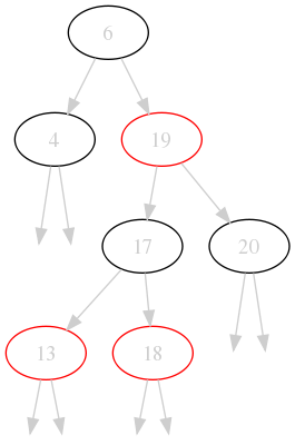
Let's look at our canonical example as it will look with an Red-Black tree as container:

Our example as red black tree

See. In a sense it is prettier than the AVL tree because it has colors! But it is also not so pretty because it is not so well balanced. But you can immediately check that the properties are fulfilled:

  • The root is black.
  • Each red node has only black children (or none).
  • There are always 2 black nodes on each path from leaf to root.

So this is indeed a valid Red Black tree.

We looked at three types of binary search trees by now and we have implementations for all three of them available. What lies closer than benchmarking them?

Benchmarking

For the following tests I used two lists of values:

  • A: the values from 0 to 2999 in random order. No duplicates.
  • B: 1000 random values in the same range including duplicates.

I measured the time to

  • insert all values from A into each container (insert column).
  • delete all values from B from the filled container (delete column).
  • search for all values from B in the filled container (search).
  • construct a sorted list - that is an inorder traversal - from the filled container (iterate).
Tree type insert delete search iterate
BS 36 ms 14.4 ms 8.49 ms 6.49 ms
AVL 117 ms 16.0 ms 6.89 ms 5.39 ms
RedBlack 64 ms 19.8 ms 6.9 ms 5.52 ms

The timings are as expected: insertion and deletions goes fastest in the binary search tree (BS) because it doesn't need to do anything special. The AVL tree is slowest because it is most aggressive with balancing the tree. It gains ground on the red-black tree on deletion though: maybe the extra work on deletion is not so bad for the AVL tree; note it is still slower than the binary search tree.

Funny enough, searching and iterating is not really much faster in the AVL tree compared to the red-black tree. That shows why red-black trees are used so often: they are an excellent trade off in insertion/deletion speed compared to search speed.

Conclusion

Today, I presented you a very, very brief look at Red-Black trees. We only talked through the properties and looked at one example. I also finished the series with a benchmark for all three implementations.

You can find the implementations in the GitHub repository of mine. Take them for a spin yourself! If you are more of the theoretical type, go devour the Wikipedia page on Red-Black trees instead.

This concludes my series on binary search trees. If I feel so inclined, I might make another tree topic about B-Trees which I find particularly interesting.

AVL Trees

The AVL Tree

Last post we looked at the Binary Search Tree in some detail and we found that it is a pretty good data structure. We also found that it behaves like a linked list and looses its good properties when we insert items in sorted order. Let's work on this and check out a tree that is auto balancing: the AVL tree.

The AVL tree is a binary search tree with one new property: in each node, the height of the left subtree and the height of the right subtree must only differ by 1 (or zero). That's all there is to it. Let's look at the binary search tree example we saw the last time and check out what needs to be done to make it a AVL tree.

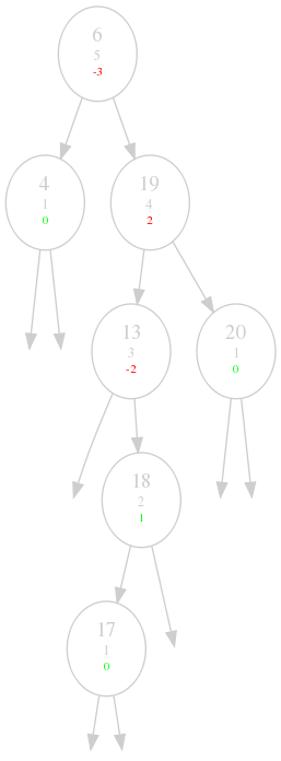
A bst with heights and height balances

The keys are still written in bigger font size, but I now added two more properties: the smaller numbers in grey is the height of the node. For a node $$n$$, with children $$l$$ and $$r$$ the height $$h(n)$$ is simply defined by

\begin{equation*}h(n) = 1 + \mathrm{max}\Big( h(l), h(r) \Big)\end{equation*}

The colored number is the height balance of a node, which is just the height of its left subtree minus the height of its right subtree. So for example the node 13 has no left subtree, so $$h(l)$$ = 0, the node 18 has height 2, so $$h(r)$$ = 2, this results in a height balance of -2. The numbers are green when they do not violate the AVL property, otherwise they are red.

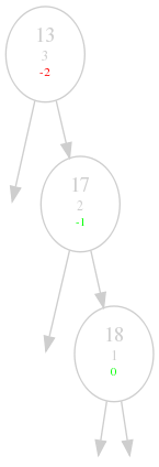
So what do we need to do to fix the 13 for example? Intuitively, we would like the 13 to go down and the 18 and 17 to come up in some kind of way. But obviously, we need to keep the ordering of the binary tree. The solution is quite simple, first, we do a right rotation with the 18 as root, then we do a left rotate with 13 as the root:

Step 1: right rotate with 18 as root
Step 1: 17 moved up and 18 moved down.
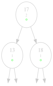
Step 2: left rotate with 13 as root
Step 2: 17 moved up and 13 moved down and everything is balanced.

So what is a rotation? For example the left rotation with $$P$$ as root looks like the following. $$R$$ is the right child of $$P$$.

  • $$P$$ becomes the left child of $$R$$
  • $$R$$'s left child becomes $$P$$'s right child

That basically means that $$P$$ comes down while $$R$$ goes up. The right rotation looks the same, but right and left swapped.

What changes for the handling of the tree? Searching and traversing stays the same, it is a binary search tree after all. What about insertion and deletion?

Insertion

Insertion is simple: we just insert the node where it belongs, but than we have to make sure that the AVL property is not violated anywhere. It isn't automatically violated after insertion, but if it is, it can only be violated in one node which is on the path we took while going down the tree. We rebalance this node and are done.

def _just_inserted(self, node):
    "Node was just inserted into the tree"
    par = node.parent
    while par:
        self._update_height(par) # Recalculate the height of the parent
        if abs(par.height_balance) > 1:
            self._rebalance(par) # Rebalance the one node and stop
            break
        par = par.parent # Otherwise continue with parent

    return node

Deletion

Deletion is also easy: The case of a node with two children doesn't change and the deletion in the other cases are just the same. But the height of all the nodes on the path we took down to the nodes might have changed, so we have to check for this and rebalance accordingly. If we encounter a node on our way up that has not changed height, we can stop checking because the nodes above it will not feel any difference.

def _delete_leaf(self, n):
    par = n.parent
    BinarySearchTree._delete_leaf(self, n)
    self._rebalance_till_root(par)

def _delete_node_with_one_child(self, n):
    par = n.parent
    BinarySearchTree._delete_node_with_one_child(self, n)
    self._rebalance_till_root(par)

def _rebalance_till_root(self, node):
    while node and self._update_height(node):
        node = node.parent if \
           abs(node.height_balance) <= 1 else self._rebalance(node)

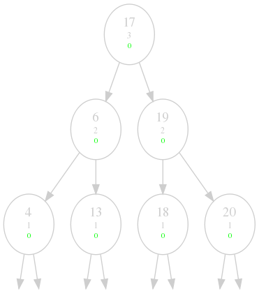
That's all there is to it. Let's repeat our ending experiment from the last time and insert our values in sorted order in our shiny new data structure:

The final AVL-Tree of our example

Perfect. But how good is it in the general case?

Number of nodes in the tree

Given $$m$$ nodes, what will be the height of the tree be like? Well, it will likely be some kind of logarithm $$m$$. Let's check this more closely.

Let's define $$n(h)$$ to be minimal number of nodes in a tree of height $$h$$. There is an easy formula for that: the smallest number of nodes is when the left subtree has an height of h-1 and the right h-2, so

\begin{equation*}n(h) = n(h-2) + n(h-1) + 1\end{equation*}

I will state that the following is true and proof it by induction later on.

\begin{equation*}n(h) \geq c^{h-1}\end{equation*}

The question is, what will the biggest $$c$$ be that still solves this inequality? Let's solve for c:

\begin{eqnarray*}(h-1) \log c & \leq & \log n(h) \\ c & \leq & \exp \Big\{ \frac{\log n(h)}{h-1} \Big\}\end{eqnarray*}

Here are some numbers:

h $$n(h)$$ max $$c$$
3 4 2
4 7 1.9129
7 33 1.7910
20 17710 1.6734
50 32951280098 1.6392698637801975

Let's do the induction finally. We assume that the condition holds for smaller values, we than only have to show that it also holds for $$n$$:

\begin{eqnarray*}n(h) & = & n(h-2) + n(h-1) + 1 \\ & \geq & c^{h-3} + c^{h-2}\end{eqnarray*}\begin{equation*}c^{h-1} \leq c^{h-3} + c^{h-2} \Rightarrow c^2 - c - c \leq 0\end{equation*}

The only positive solution of this quadratic equation is the golden ration:

\begin{equation*}c_{\max} = \frac{1 + \sqrt{5}}{2} \approx 1.618\end{equation*}

Let's assume we have a tree with height $$h$$ and $$m$$ nodes in it. Now we know:

\begin{eqnarray*}m \geq n(h) &\geq & c_{\max}^{h - 1} \\ \Rightarrow \log_{c_\mathrm{max}} n(h) + 1 & \geq & h\end{eqnarray*}

And because the $$\log$$ function is monotonous:

\begin{equation*}h \leq \log_{c_\mathrm{max}} m + 1\end{equation*}

Pretty well balanced it is, indeed.

Conclusion

We continued our investigation of binary search trees and looked at a self balancing version of it, the AVL tree. We discussed the basic principle of how it works without going into all the individual cases one would encounter when deleting or inserting (you can find them elsewhere). We also looked at code that implement the differences compared to the normal binary search tree.

More information is of course on Wikipedia. The proof of height was stolen from the computer science lectures by Dr. Naveen Garg about AVL trees, he does a great job of making things clearer.

Remember, there is source code for this post on github. I added an implementation of an AVL tree that derives from an ordinary binary search tree and only implements the additional stuff we talked about.

Next time, we will look at Red-Black Trees.

Binary search trees

The binary search tree

Let's suppose you want to keep some data in memory. Occasionally, new items arrive, old items get unimportant and you want to delete them. Adding new items and deleting old should not take long. And you want to be able to traverse the data quickly and in sorted order at all points in time.

Arrays are out, because they would shuffle all the elements around on deletion and insertion. What data structures would you use?

Why not use a binary search tree? It only needs $$\mathrm{O}(n)$$ space and insertion and deletion take on average only $$\mathrm{O}(\log n)$$ time. A pretty good deal?

What is it?

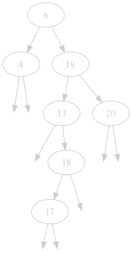
A sample binary search tree

This is one for integers. You can put everything that can be ordered inside a binary search tree, but for simplicity, we will stick with integers.

Our tree has 7 nodes in it, so $$n = 7$$. The root node is 6. See the nodes 19 and 6? They have 2 children: left and right. All nodes also have a parent. There are other nodes with either a left or a right child. There are also some nodes without any children, they are called leafs of the tree.

This is called a binary tree because every node can only have a maximum of two children. But what makes it a binary search tree? If you look closely, you will realize that all children that are to the left of a node are strictly smaller and the reverse for the right site. Look at the 19: 20 is to its right and bigger, 6, 4, 13, 18, 17 are to its left and strictly smaller. And that's all there is to it.

Searching & Insertion

This property makes it easy to check if a value is inside our tree. For example, if you want to know if 12 is in the tree you do the following:

  • Start at the root: 12 > 6 so go right,
  • 12 < 19 so go left
  • 12 < 13 so go left again... Ups.

There is no node here. Well, 12 is not in our tree, is it? But if you would want to insert it, you would do it right here, as left child of 13.

Let's look at the python code for those two operations:

def search(node, key):
    if node is None: return None
    if node.key == key: return node
    return search(node.l, key) if key < node.key else \
           search(node.r, key)

search(root_node, 12)  # None, for our case

def insert(node, key):
    if node is None: return Node(key)

    if key <= node.key:
        node.l = insert(node.l, key)
        node.l.parent = node
    else:
        node.r = insert(node.r, key)
        node.r.parent = node
    return node

insert(root_node, 12)

Note that we also do some house holding that the links between children and parents are valid after insertion.

Deleting

Deleting an item is a bit hairy, but there are only three cases:

  • Delete a leaf: Just remove it and you're done. Remember to break the links to its parent though!
def delete_leaf(n):
    if n.parent.l == n:
        n.parent.l = None
    else:
        n.parent.r = None
  • Delete a node with one child: we essentially remove this node from the chain by linking its parent to its child.
def delete_node_with_one_child(n):
    child = n.l or n.r

    if n.parent.l == n:
        n.parent.l = child
    if n.parent.r == n:
        n.parent.r = child
    child.parent = n.parent
  • Delete a node with two children. This is the most difficult one. Look at 19, how could you remove this from the tree? Well, we have to keep the ordering property. So the only two values that we could use in this position that would keep the property are 18 and 20. Those are the biggest item in its left subtree (18) and the smallest item in its right subtree (20). And this is always the case! Which one should we pick? It doesn't matter, but picking one at random will help distribute the items in our tree evenly.

    Now all that is left to do is to delete the node we took the value from.

import random

def biggest_successor(node):
    if node.r:
        return biggest_successor(node.r)
    return node

def smallest_successor(node):
    if node.l:
        return smallest_successor(node.l)
    return node

def delete_node_with_two_childs(n):
    child = smallest_successor(n.r) if random.choice((0,1)) == 0 \
            else biggest_successor(n.l)

    n.key = child.key
    delete_node(child) # could have one or zero children

Traversing the Tree

Now how about getting at the elements in sorted order? We would need to start at the leftmost element in the tree because it is the smallest. The next bigger one is the smallest element in its right subtree. We can express this in a recursion quite nicely:

def iter_tree(node):
    if node.l:
        for k in iter_tree(node.l):
            yield k

    yield node

    if node.r:
        for k in iter_tree(node.r):
            yield k

list(root_node) # -> [4, 6, 13, 17, 18, 19, 20]

Is it a deal?

So we have a nice data structure now, should we use it? Yep. Can we achieve better? Not in the average case. Is is good for all cases? Well, just imagine your data arrives already in sorted order:

Tree becomes a link list on sorted insertion
Rotated to save some space. And it sorta looks like a linked list.

Terrible! Gone is our $$\mathrm{O}(\log n)$$ search time (it is $$\mathrm{O}(n)$$ now). And with it the nice performance of inserts and deletions. What can we do about it? There are some more advanced trees that are able to keep themselves balanced, that means that there are around the same number of nodes in each subtree of each node. We will look at AVL Trees and Red-Black Trees in future installments of this series.

Conclusion

We took a quick glance at binary search trees, how they work and why they are useful. We discussed how easy insert is and that deletion is quite straightforward, but there are many different cases. We also looked at python snippets that implemented the functionality we talked about.

If you want to know more you can either hop over to Wikipedia and read it up for yourself. Or, you can watch the excellent computer science lectures by Dr. Naveen Garg about data structures - especially trees.

Or you could check out the source code for this post on github. There you will find my implementation of a binary search tree and also the visualization routine I used to make the images of our tree here.

Anonymous snippets in UltiSnips

Anonymous Snippets in UltiSnips

UltiSnips supports anonymous snippets: they are defined on the spot, expanded and immediately discarded again. They were requested by someone and Ryan implemented them, but I was all Meeeh because I didn't understand for what they could be used.

But I just realized they are in fact awesome: I have a new line in my RestructuredText Vim plugin file:

inoremap <silent> $$ $$<C-R>=UltiSnips_Anon(':latex:\`$1\`', '$$')<cr>

Hitting $ now directly translates into being in inline math mode. How cool is that?

The de Casteljau Algorithm

The de Casteljau Algorithm

This is a follow up to Blender and Blossoms.

The de Casteljau Algorithm is a recursive way to calculate the Point on a Bézier curve given its control polygon $$P = \{ \vec{b_i} \}$$ consisting of the Points $$b_i$$. It is defined as follows in the Book:

Given the points $$\vec{b}_0 ... \vec{b}_n$$, $$t \in \mathbb{R}$$ and a function $$f(t): \mathbb{R} \to \mathbb{R}$$. Set

\begin{eqnarray*}\vec{b}_i^0 & := & \vec{b_i} \\ \vec{b}_i^r & := & (1-f(t)) \vec{b}_i^{r-1} + f(t)\,\vec{b}_{i+1}^{r-1}(t)\end{eqnarray*}

Then $$\vec{b}_0^n$$ is the point with the parameter $$t$$ on the corresponding Beziér curve.

So this is essentially a recursive definition: Starting from $$n$$ points, we always combine two of them and remain with $$n-1$$ points. We continue this scheme until only one point is left. This is the point on the curve for the value $$t$$.

Implementation

The de Casteljau Algorithm is short and beautifully implemented:

import numpy as np

class DeCasteljau:
    def __init__(self, *pts, func = lambda t: t):
        self._b = np.asarray(pts, dtype=np.float64)
        self._func = func

    def __call__(self, t):
        b, n = self._b, len(self._b)
        for r in range(1,n):
            for i in range(n-r):
                b[i] = (1-self._func(t))*b[i] + self._func(t)*b[i+1]

        return b[0]

And this is how it looks.

Blender screenshot of polygon with bezier curve

The orange curve is the defining polygon and the dots are the corresponding beziér curve evaluated for 100 values of $$t \in [0,1]$$ and $$f$$ being the identity.

You can find the complete code in the GitHub repository under chap04.

New parser for UltiSnips

UltiSnips got a new parser

UltiSnips is the Vim plugin for Snippets I have started. It has become fairly successful with quite some people contributing snippets and code to it. I use it myself on a daily basis and can't remember how I did things before it was around. For example, I have the following snippet defined to start blog posts:

snippet blog "Blog Post Header" b
---
uuid: `!p if not snip.c: snip.rv = uuid.uuid4().hex`
date: `!p snip.rv = dt.datetime.now().strftime("%Y/%m/%d")`
type: ${1:article|quote|link|image|video|audio|custom}
title: ${2:Awesome, but short title}
tags: ${3:tag1,tag2}
---

${0}
endsnippet

The first line introduces this as a snippet definition, while the last line ends it. All between is pasted into my text when I type blog followed by a <Tab>. There is some special syntax:

  • The parts starting with backticks are python interpolated code; that is the first line will become a UUID, the second the current date.
  • The parts starting with ${<number> are tabs. They get selected and when I expand the snippet. I overwrite them my own text, then, by pressing <C-j> I quickly jump to the next tab which is then selected so I can overwrite it.

In toto, UltiSnips spares me to remember a lot of Syntax (like the various article types my blog supports) and a lot of manual work (like putting in the date or creating a UUID). I love it.

The purpose of parsing

When <Tab> is pressed, UltiSnips must learn where the snippet needs to be inserted and where the individual Text Objects (tabs, python code, shell code, vimL code, mirrors, transformation or escaped chars) end up in the text file the user is writing. This needs to be done by learning first where the text objects are inside the snippet and how they relate to each other (e.g., tabs can also be inside default text of other tabs). For this, parsing of the snippet is needed.

The original approach was to use a bunch of regular expressions to find individual Text Objects inside a snippet. This has a number of downsides, the two biggest are that

  • the snippet syntax is not regular.
  • the snippet syntax may contain ambiguity

See this example:

$1 ${1:This is ${2:a default} text} $3 ${4:another tabstop}

The first point is exampled by the 1 tabstop: regular parsing is out of the picture here, because you need to count the { and } to make sure you do not take too little or too much text into your tabstop.

The ambiguity is with the $<number> syntax: The first $1 is a Mirror (a text object that simply repeats the contents of a tabstop), because a tabstop definition appears later in the snippet. The $3 however is a tabstop without default text as there is no proper tabstop definition for 3, so the $3 could be replaced via ${3:} or ${3} and the snippet would behave exactly the same.

Never the less, we had a regular parser for a while now and jumped through many rings to support the cases I just mentioned. Not any more.

The new approach

This the what the new algorithm does:

  1. Tokenize the input text with a context sensitive lexer. The lexer checks for each position in the string which token happens to start here. If one potential token is found, it is parsed according to its own rules.
  2. Iterate through all tokens found in the text.
    1. Append the token and its parent to a list of all tokens in the snippet. As we recurse for tabstops (see next point) this builds a list of tokens in the order they appear in the text.
    2. If the token is a tabstop, recurse the algorithm with text being the default text of the tabstop and parent being the tabstop itself.
    3. If the token describes a text object that has no immediate reference to other tabstops (e.g. Python code interpolation, shell code interpolation or escaped special characters) create the text object and link it to its parent.
  3. When the whole snippet is traversed, do the finalizing touches for the list of all tokens and their parents:
    1. Resolve the ambiguity. As we have seen all tokens by now and already instantiated all easily identifiable tabstops we can go through all the $<number> tokens in order and decide if they are a tabstop (first appearance) or a number (a tabstop is already know for this number) and create them accordingly.
    2. Create objects with links to tabs. Transformations take their content from a tabstop. Now, since all tabs are created, we can traverse the list of tokens again and create all the transformations and pass them their proper tabstop. Also, only now can we detect if a transformation references a non existing tabstop.

You can find the implementation of the new parser in the _TOParser class and the implementation of the lexer in the new Lexer.py file.

Adding discussions to the blog

Discussions using Disqus

I just introduced a new feature to this blog which is something I wanted to have for a very long time: Discussion threads. I already talked about this in my original revamping the site article and I basically went with what I have had planed.

So this site is now using the Disqus service for handling comments. This means you can use basically any account you already have to comment on my work here on the blog or just comment anonymously. I wonder how good the spam handling of Disqus is.

Implementation

From an implementers standpoint, the Disqus API is very straightforward and well documented. Essentially you just define some javascript variables, then include some scripts from disqus.com in your site and you're done.

The control is not as fine tuned as I would have liked though. For example you do not get the chance to iterate over every comment and output your own HTML code. I do not doubt that it is possible by looking at the javascript from Disqus, but it is not officially supported.

Style

However, the wonders of CSS gave me the power to reformat their HTML output to match the prettiness of black and yellow. I had to redefine some formatting that where already set by my styles - then overwritten by the Disqus style sheet for their elements - to match my style again. A little cumbersome, but easy.

I mostly looked at the rendered page source to figure out which classes I needed to format in the CSS, but there is also a nice blog post on onbloggingwell.com on this very topic which was useful.

So, I hope to read some comments in the future! I will go ahead and make the first test post as anonymous myself right away, you can bet on this :).

Blender 2.5 and Blossoms

Using Blender 2.5 as Visualization Tool

For my PhD work I use Blender as visualization tool. It suits me because it uses python for scripting and is very flexible. I can also use it directly to navigate my results and render them for publication.

Blender has seen a major overhaul with version 2.5, nearly everything works differently: the GUI has changed, the internal python API has changed, the feature set has changed (grown mostly). Getting my stuff from Blender 2.4 to Blender 2.5 will be a major undertaking which I do not want to tackle now. However, I feel that it is about time to start learning it, because before I give my work to my successor, I should really port it to the current blender version.

Reviewing Interpolation

Also for my work, I am currently skimming through the book Curves and Surfaces for GACD by Gerald Farin. I need some inspiration for a better representation of my surfaces. It is a great book. If you are interested in programming 3D graphics or interpolation you should really get it.

The programming problem P1 in chapter 3 is the following:

Let three points be given by

$$$\vec{b}_0, \vec{b}_1, \vec{b}_2 = \begin{bmatrix}0 \\ 0\end{bmatrix}, \begin{bmatrix}40 \\ 20\end{bmatrix}, \begin{bmatrix}50 \\ 10\end{bmatrix}.$$$

For s = 0, 0.05, 0.1, ...1 and t = 0., 0.05, 0.1, ..., 1 plot the points b [s,t].

The function b is defined earlier in the book and is called a bivariate Blossom. It is defined by the following equation:

$$$\vec{b}[s,t] = (1-t)(1-s) \vec{b}_0 + [(1-t)s + t(1-s)]\vec{b}_1 + s t \vec{b}_2$$$

Using the brevity of Python, this results in this wonderful class definition:

 1
 2
 3
 4
 5
 6
 7
 8
 9
10
11
12
import numpy as np

class Blossom(object):
    def __init__(self, p1, p2, p3):
        self._pts = np.asarray([p1, p2, p3])

    def __call__(self, t, s):
        return np.dot((
            (1-t)*(1-s),
            (1-t)*s+t*(1-s),
            s*t),
            self._pts)

Putting it together

So I put together a python script that can be loaded and executed in Blender 2.5. It sets up a menu that is shown in the 3D View whenever a mesh with exactly 3 vertices is selected. It allows you to set the range for s and t and updates the Blossom mesh with the calculated points.

The final result looks something like this:

the menu is on the left, the Polygon and the Blossom is on the right

It took a while to put the script together: The documentation of the new python API is not very complete at the moment and googling for Blender 2.5 specific help is not trivial. I hope this script gets someone else jump started. You can find the python script here and the blender scene which also includes the python script here.

Update: The code is now also available on GitHub.

Revamping the site

Revamping the site

Welcome back to my new and drastically improved website! In the last few weeks I worked to improve all aspects of the site for my own benefit mostly, but also for yours! So what you see here is all new: new design and new deployment technology. Only the content hasn't changed.

New Technology

Okay, I didn't blog as much as I wanted to in the past. There were numerous reasons, but lack of content wasn't the dominating one. The biggest problem was that the old django site didn't allow to quickly write down and preview a blog post in Vim. There was always a mental barrier to get started writing my thoughts down.

So I switched from Django to Blogofile which is basically a fancy static web site generator written in Python. So instead of generating the HTML on the fly on the server it is generated offline and then uploaded to the server. This has a number of advantages like enhanced security, quicker deployment and serving of the site. It also means I have the whole site under version control at all time and can carry it around with me wherever I go.

The disadvantages is that there is no longer any dynamic behaviour on the server site possible, so no fancy session support or contact forms. I have some ideas how this could be monkey patched into this, but for the moment I can live without that. I also believe that there is quite a lot possible with using javascript, so I might not need server site scripts at all.

The site is basically at the same functionality level than the Django site I used before. Especially code and LaTeX integration are top notch (for me). We still have no comments, but I hope to get Disqus Integration rolling sometime soonish.

New Layout

I was a bit sick of my old layout. It was ugly. The reason it was ugly is that I have no skill with CSS and HTML. Yep, I know the technical parts of it, but I am not a good designer, have no eyes for fonts, colors and so on. So I decided to spend some bucks and support a freelancing designer named kubasto on themeforest.

I personally find the dark black-yellow design gorgeous. And kubasto knows his trade: He included some javascript snippets to integrate with twitter, facebook and what not. I had some work to do to convert his code from PHP back to Mako Templates, but I think I have ironed out the most awful bugs by now.

What's next?

I revamped the blog for a reason: I finally want to do what I promised to do when I started this thing. I also need a page for some of my personal projects (e.g. UltiSnips) and as I am currently revamping a lot of topics from statistics, machine learning and computer science I want to provide short blog posts with explanations and code for others (and myself in a few years) to follow and learn from. Let's hope I deliver this time!

Zsh niceties

Zsh niceties

I am using the zsh forever now, today I stumbled upon mikas advent calendar where he lists a lot of zsh niceties. I list some of them here so that I can find them later on. All below is me paraphrasing nikas wisdom. You obviously want to put most of this into your .zshrc.

Hashes

Hashes are very useful shortcuts:

$ hash -d prog=~/Desktop/Programming
$ cd ~prog # or just ~prog

Edit-command-line

This one is most useful too! Add the following lines to your .zshrc and in the future, just hit Esc-e to edit your current command line.

in your $EDITOR:

autoload -U edit-command-line
zle -N edit-command-line
bindkey '\ee' edit-command-line

vcs_info

I haven't heard before of vcs_info before, but if you use git or mecurial, this one is really valuable. It is also mighty slow with bzr and might clobber your console with debug output, but give it a try. You need to adjust PS1 to your needs.

autoload -Uz vcs_info
zstyle ':vcs_info:*' disable cdv darcs mtn svk tla

precmd() {
  psvar=()
  vcs_info
  [[ -n $vcs_info_msg_0_ ]] && psvar[1]="$vcs_info_msg_0_"
}

PS1="%B%(?..[%?] )%b%n@%U%m%u%(1v.%F{green}%1v%f.)> "

globbing

I tend not to use globbing this much, except for the usual stuff like ls */**/*.py or so, but zsh's globbing features are definitively worth a checkout.

Me@26c3

26c3 in Berlin

As usually, I am at the Chaos Communication Congress in Berlin between the years together with huega. We are a quite reduced number of people this year for various reasons: The first one is that most of our direct friends chickened out and stayed at home. The second reason is that the CCC did put a hard limit on tickets sold this year. This is sad, because not everybody that came to Berlin could attend, but this is also good because the congress is not totally overcrowded: You have a chance to attend the talks you are interested in and occasionally you get a place to sit down and hack for a bit.

I did various things on the congress already:

  • I invested some time in lua and learned how to embed it into C/C++.
  • I continued my work on fbuild (link to new GitHub page) and wrote a cython builder for it. It still sucks, that's why you can't find it yet on the internet. Eric was so nice to implement some features which made my life much easier.
  • I made a MiniPov V3 and learned how to use the AVR toolchain. This is quite impressive: The processor has more potential then the PICs I currently use for my projects and the tool chain is easier to use. To get acquainted with it, I wrote a software PWM that made the LEDs on the MiniPov fade in and out. This took less than 30 minutes. Impressive!
  • I finally took some time to pimp my blog. See previous post. Hopefully this will push me to more often post some content here.

Okay, enough chit-chat. Next talk is coming up.

Oh, here is a picture of me happily hacking away taken by huega. And another of me waving my brand new MiniPOV.

me @26c3me waving my MiniPov
Some new tricks

Teaching the blog some new tricks

Year, I know. This blog is not really used as often as I hoped I would. I have quite some material on my hard drive and in my brain that I'd like to dump here: Example scripts for science, some django stuff and so on. But for now, at least one new post: I've taught the blog some new tricks. Let's go through them one by one.

1 Restructured Text

The first thing was that I changed away from markdown syntax for my entries to RestructuredText. The reason for this is pretty simple: I prefer the syntax (it is much easier to read in text form) and it offers more flexibility. What kind of flexibility? Read one.

2 Support for code snippets

Following along the lines of Josh VanderLinden's excellent post I implemented syntax highlighting using pygments. This allows me to show code snippets in various languages, like for example python:

k = "hello world"
print k.title()

Or for example LaTex:

e^{i \pi} + 1 = 0

I like it a lot, this will make posting programming stuff a lot easier.

3 Latex support

The last new trick I want to rant about is LaTeX support. For example, the above formula looks like this in the blog:

$$$e^{i \pi} + 1 = 0$$$

Those three changes all together will make it a lot easier to post about scientific stuff in the future. Let's see if I do it this time.

GMX SMS Sending script

The Woes of SMS

So GMX decided they wanted to become more secure. For whatever reasons, this is always good thinking. But in the process of changing their Email login, they also seem to have turned off the old SMS service that I was happily using for years to pump my SMS out.

So with this option lost, I started looking for alternatives. There is no official support from GMX for SMS outside windows. I found GSMS which seemed like something I wanted, but not quite (no encryption and quite slow to send, need the user to set the GMX skin to the old style, otherwise it won't work). I also found a Perl script in a forum, but I lost the address. Both tools use the same technique: Pretending to be a browser and clicking through the site.

I did my own version. It uses the same technique, but is threaded so crawling can happen in the background. Here is the feature list:

  • Comes with address book plugin for Mac OS X
  • Crawling happens in the background, so you can start entering your SMS right away
  • SSL encrypted transport. We're not in the nineties anymore...
  • Written in python

Code

You'll find all code here: /code/GMXSmsSend. This is also a bazaar repository, so you can get the latest version or branch from it:

$ git clone https://github.com/SirVer/GMXSmsSend.git

The program needs pyqt as a GUI and obviously BeautifulSoup as a HTML parser. That's it.

Getting it to run

Edit Sms.py and add your username and your login. You can then directly run the script:

$ ./GMXSmsSend.py

Installing it as a AddressBook Plugin

Copy the file Send GMX SMS.scpt to the folder ~/Library/Address Book Plug-Ins/. Create the folder if it doesn't exist. Restart AddressBook. You might want to edit the script in case the path to python is not correct, which is quite likely the case. That should be it. If you now click on a mobile number in AddressBook, you can choose to send a GMX SMS. You will then asked for the path to the program SendGMXSMS. Point this to your created application. From now on, this should work automatically.

If you have any problems, feel free to contact me.

Blogging tryout

Let's get this started

Well, after a long time of being a computer geek, I finally decided to start a blog. The reasons for this and everything you need to know about me can be found in the about section of this page.

The engine of this page is using django. I decided to use a web framework since I never ever wanted to write pure HTML again after I left school. Django is written in my favorite language python and therefore allows me fast expansion of functionality. Occasionally, I might write some clues for working with it on this very site.

There is still a lot missing on this site. No comments, no search, no tagcloud. I might add some of this stuff, but the site is now in a state where it can help me to dump my brain. I will invest more time into it, if it shows that I really use it.

Alright, the basics are done, the engine is ready. Let's see where this blogging stuff leads us...