Least squares
Here we go again. After a long time of travelling and illness something new on this blog. Today, I start a new mini series that takes a look at Least Squares in various ways. I want to show how least squares arises naturally in various areas - of course this will look at little similar all the time because it stays the same principle; but the basic approach depends on the context.
Today we start with a simple example and the method I'll call the direct approach.
The direct method
Suppose we have some kind of measurement process that measures every second and we know that the system we measure follows a model of third order, that is the values we expect are
But obviously, our measurement process is in some way noisy. Our aim is now to find good values for $$p_1, p_2$$ and $$p_3$$. But what is good? Well, why not start by minimizing the distance between our model prediction and the measurement values?

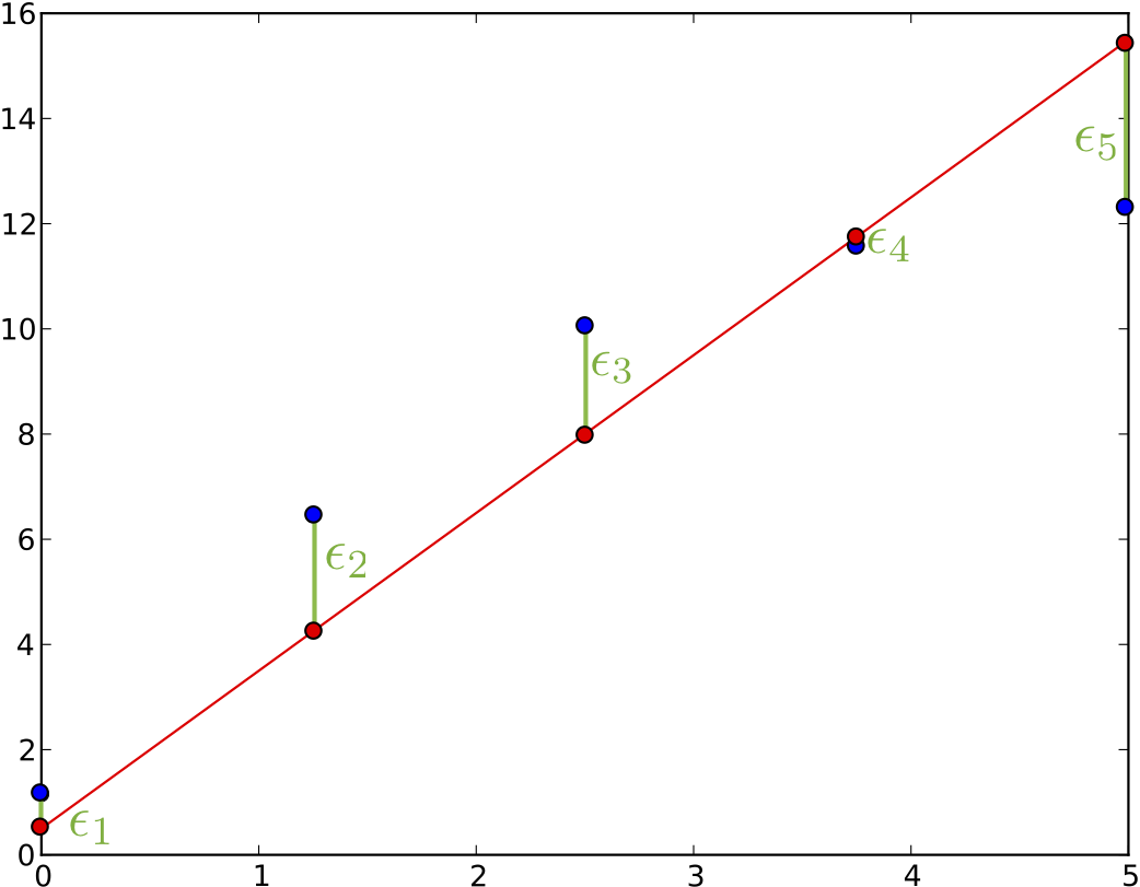
In this plot we see our measurements as blue dots and we see an awful model fit as red line. And we see various $$\epsilon$$ bars. Those are the errors we want to minimize, the model prediction at a point $$t_i$$: minus the value that we measured at this point $$v_i$$:
It seems like a bit of a stretch to write this simple equation in a matrix notation there in the last step. But it will benefit us in a moment.
We do not want to minimize the straight sum of those because positive and negative values might zero out. The absolute value is also not so easy because our error function is then non-smooth... Let's summarize the sum of squares of the individual errors:
Minimization is best when we have a quadratic error function because there is only a single global minimum which can be found by setting the gradient to zero.
The notation of this minimization becomes a bit tedious, that's why we go back to the matrix notation we used earlier and realize that we can stack all measurements we have into one matrix. Working with vectors will make the derivatives easier to do:
Our error function $$S$$ then becomes
Finding the gradient of S with respect to the parameter vector $$\vec{p}$$ is now easy. We also immediately set this equal to the zero vector to find the minimum of this function:
And so we find the parameters that minimizes the error to be
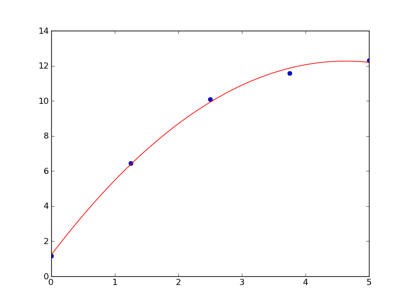
Using this with the above example we get the following best fit

Conclusion
I call this the direct approach because we directly set out to minimize the quantity and the least square formula pops out. There are other goals one can set out to achieve which leads to the same formula which I will show in some of the next posts. Hopefully it will not take as long again till I find some time to post again.
